Custom analysis of scRNA-seq data with CytoTRACE
- The gene expression table should be unfiltered and unnormalized with cells as columns and genes as rows.
- Phenotype tables (optional) must contain two columns where the first column is single cell IDs and the second column is the phenotype labels. Please do not include a header.
Dataset integration input
Pre-computed results
Differentiation status by phenotype
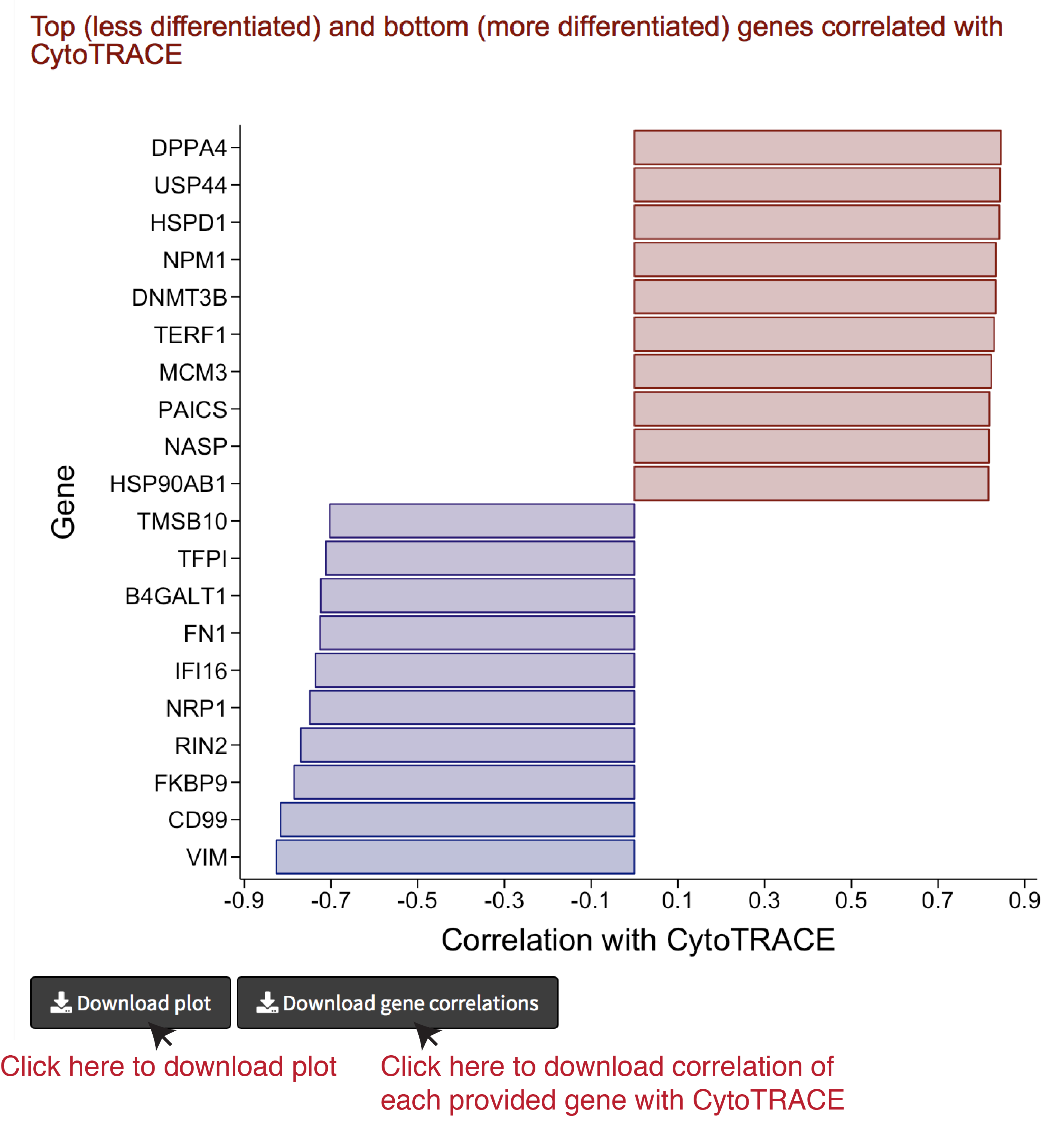
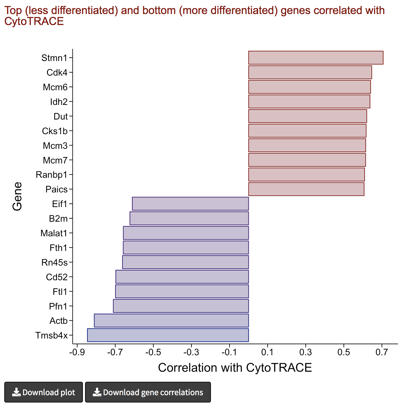
Top (less differentiated) and bottom (more differentiated) genes correlated with CytoTRACE
Overview of CytoTRACE
CytoTRACE framework
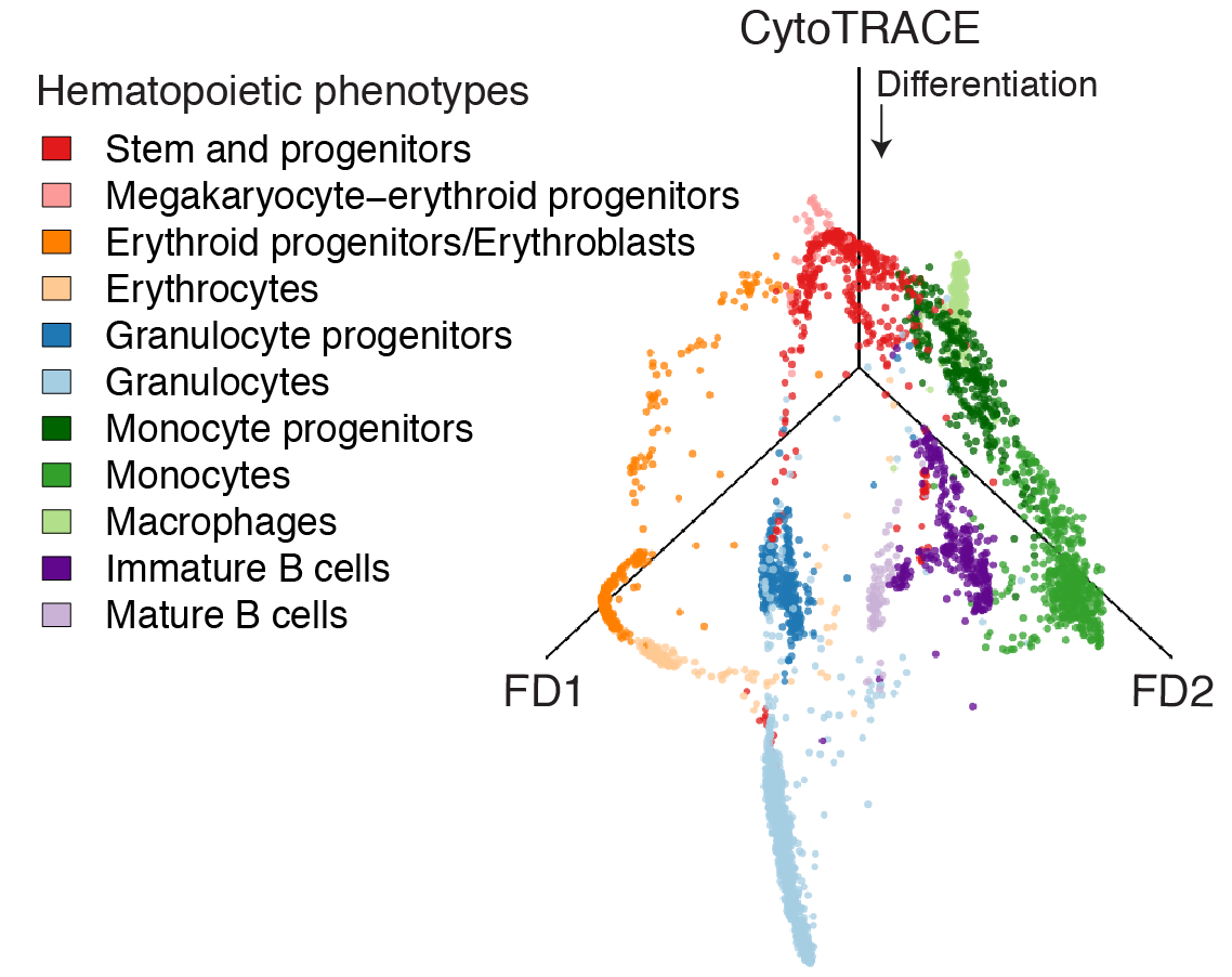
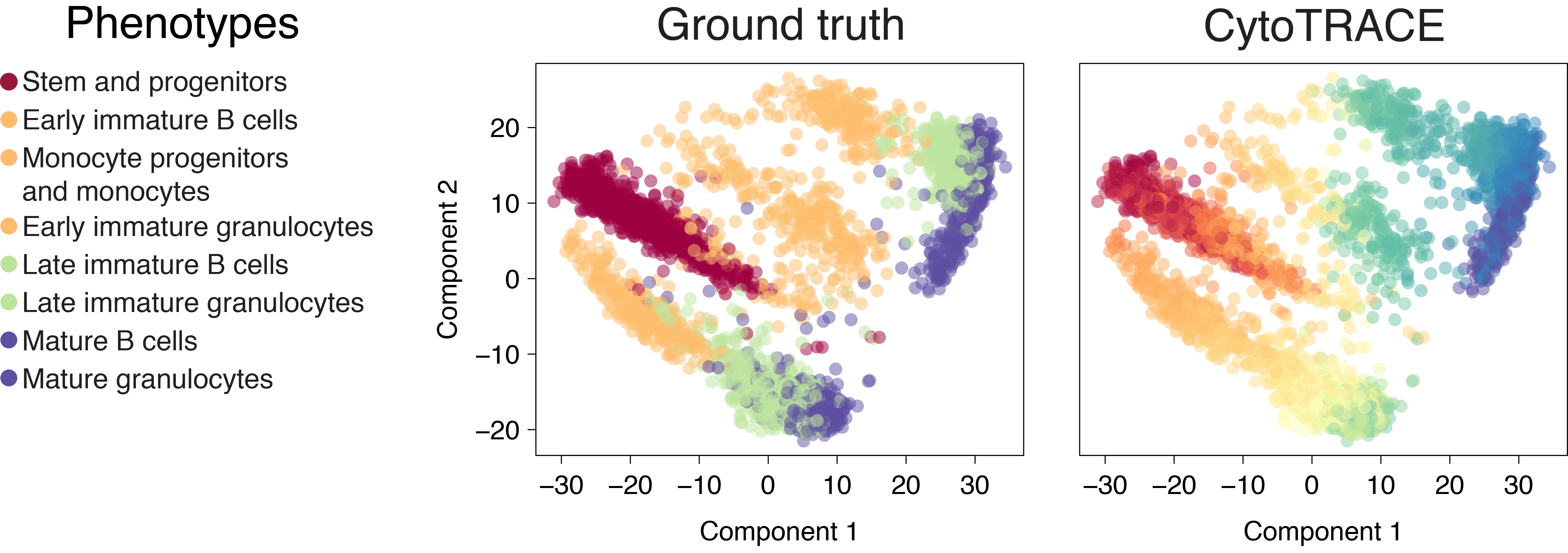
CytoTRACE prediction of bone marrow differentiation
Website features
- Analyze 42 publically available, annotated scRNA-seq datasets pre-computed with CytoTRACE
- Predict differentiation states in a custom scRNA-seq dataset
- Predict differentiation states across multiple batches/datasets from different platforms and developmental stages
- Visualize predicted differentiation with an interative 3D graph (includes t-SNE, force directed layout, and UMAP)
- Summarize results by known phenotypes
- Identify predicted stemness- and differentiation-associated genes
Examples
C. elegans hypodermis and seam (10x)
C. elegans muscle and mesoderm (10x)
C. elegans ciliated neurons (10x)
C. elegans duct and pore (10x)
Early zebrafish (Drop-seq)
Bone marrow (10x)
Bone marrow (Smart-seq2)
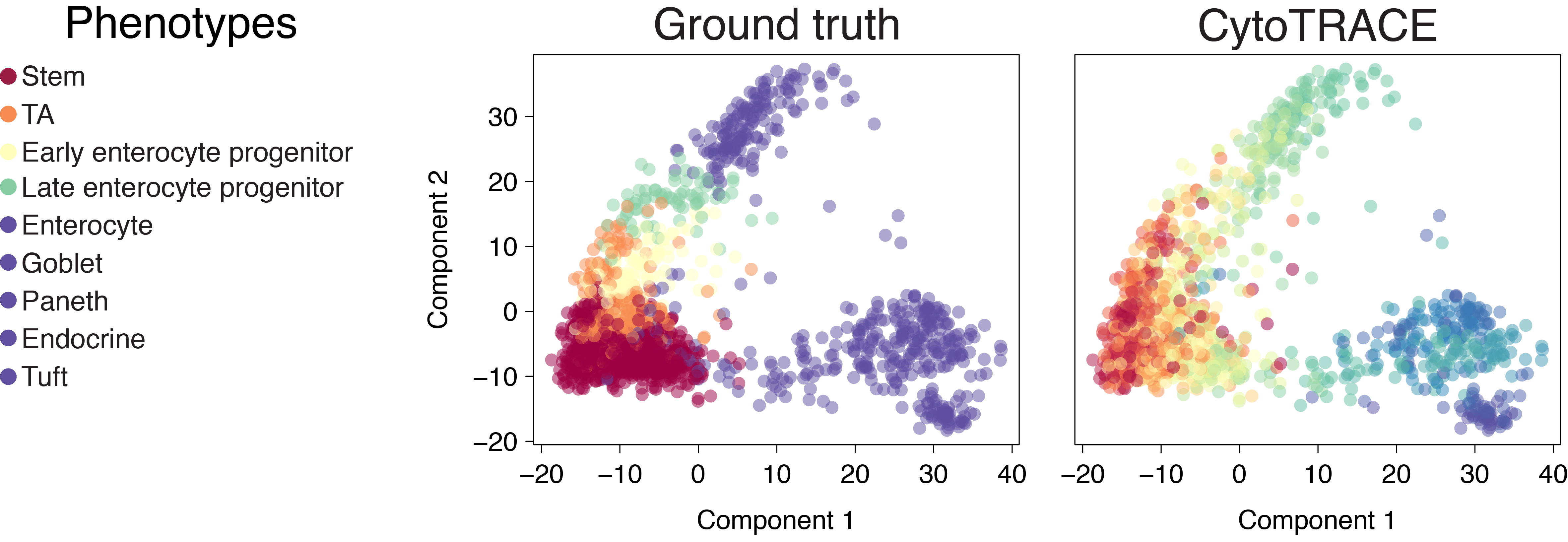
Whole intestine (Smart-seq2)
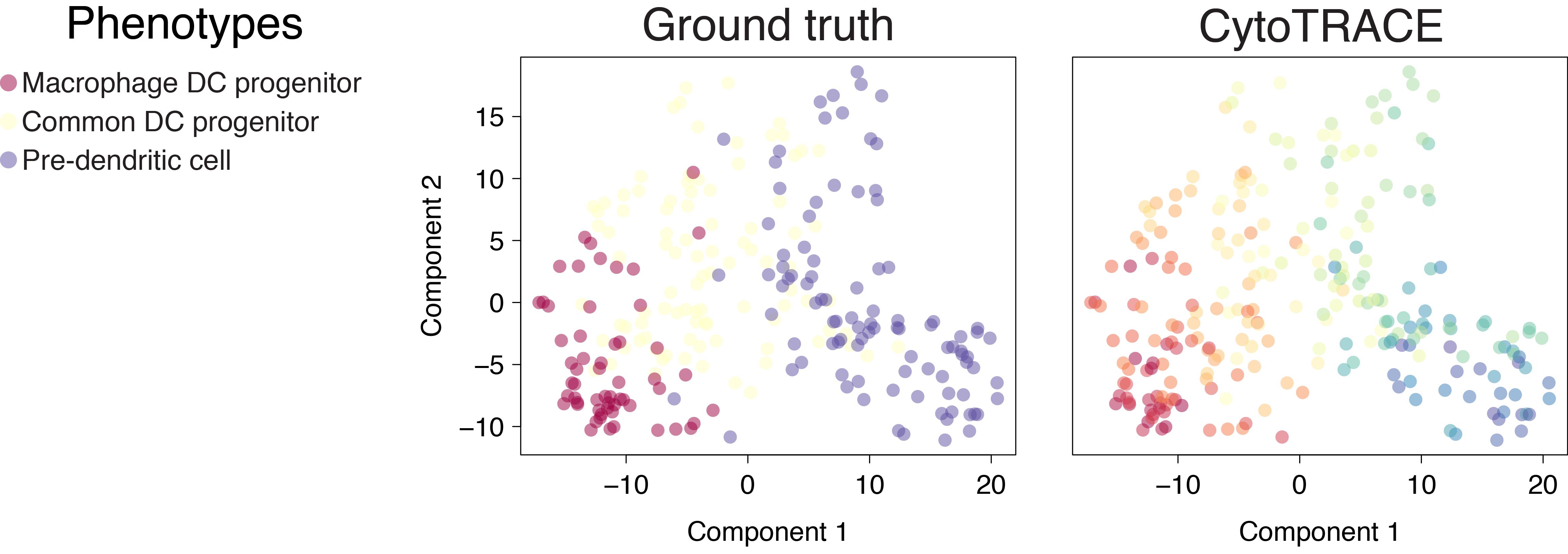
Dendritic cells (C1)
Frequently asked questions
- What is CytoTRACE?
- Why should I use CytoTRACE?
- How does CytoTRACE work?
- What do I need to run CytoTRACE?
- How should expression data be normalized?
- My data appears to be too large to analyze on the website. What is the file size limit to run CytoTRACE on the website?
- I have data from multiple batches. Can I still run CytoTRACE?
- Does CytoTRACE work with different platforms, tissues, and species?
- Are there situations where CytoTRACE may not work?
- CytoTRACE leverages single-cell gene counts. How does sequencing depth, drop-out, and other technical factors in scRNA-seq data affect the number of detectably expressed genes?
- I still have so many questions, is there someone I can reach out to for help?
What is CytoTRACE?
CytoTRACE (Cellular (Cyto) Trajectory Reconstruction Analysis using gene Counts and Expression) is a computational method that predicts the relative differentiation state of cells from single-cell RNA-sequencing data. It is capable of inferring the direction of differentiation without any prior knowledge and is robust to differences in dataset characteristics, e.g. tissue type, scRNA-seq platform, and species. CytoTRACE leverages a simple, yet robust, determinant of developmental potential—the number of detectably expressed genes per cell, or gene counts. We have validated CytoTRACE on ~150K single-cell transcriptomes spanning 315 cell phenotypes, 52 lineages, 14 tissue types, 9 scRNA-seq platforms, and 5 species.
More information on why you should use CytoTRACE and how it works is provided below.
Why should I use CytoTRACE?
CytoTRACE was developed to predict differentiaton states in scRNA-seq data without any prior information. Some examples where CytoTRACE may be useful, include:
Validating differentiation states in tissues with functional evidence of developmental states
Predicting differentiation states in human tissues where developmental hierarchies are poorly understood
Predicting differentiation states in diseased tissues, such as cancer
Identifying cells and genes associated with stemness and differentiation
Associating cancer cell differentiation states with survival, metastasis, response to therapies, and other clinical outcomes
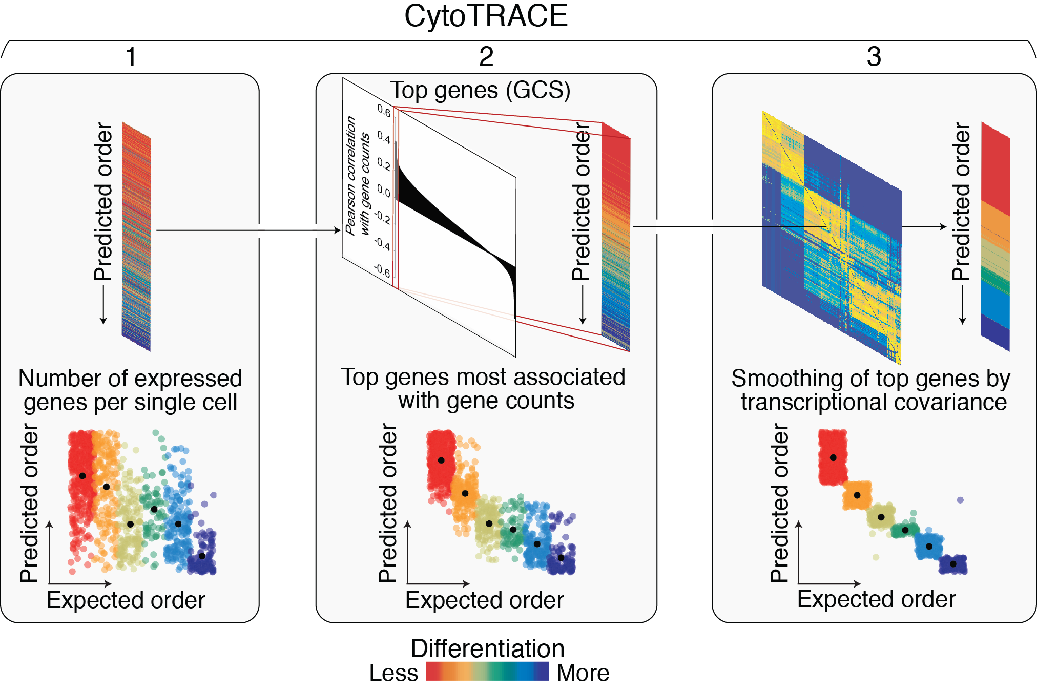
How does CytoTRACE work?
(1) Gene counts: The first step is to calculate the number of detectably expressed genes per single cell. This is done by summing the total number of genes with greater than zero expression for each single cell.
(2) Gene counts signature (GCS): The second step is to capture the genes whose expression patterns correlate with gene counts. This is done in the following steps:
First, the input gene expression table is rescaled to transcripts per million (TPM) or counts per million (CPM).
Then, the total sum of transcripts for each single cell is set to the total number of detectably expressed genes in that cell. This is done to convert the gene expression matrix to relative transcript counts, or the estimated abundances of mRNA molecules in the cell lysate, which we and others have shown to improve the detection of differentially expressed genes (Gulati et al., 2020; Qiu et al., 2017).
The resulting expression matrix is log2-normalized with a pseudo-count of 1.
To measure each gene’s relation to gene counts, the Pearson correlation between each gene’s normalized expression and gene counts is calculated.
Finally, the geometric mean expression of the top 200 genes most positively correlated with gene counts is gene counts signature (GCS).
(3) CytoTRACE: The final step is to iteratively refine our estimate of the GCS vector by leveraging the local similarity between cells and applying a two-step smoothing procedure:
First, to create our nearest neighbor graph, we convert the normalized expression matrix (see above) into a Markov process that captures the local similarity between cells.
Using this Markov matrix, we then apply non-negative least squares regression (NNLS) to GCS. This allows us to represent GCS as a function of the distinct transcriptional neighborhoods captured in the Markov matrix.
Next, we apply a diffusion process to iteratively adjust GCS based on the probability structure of the Markov process. Note: This is not GCS but an NNLS-adjusted GCS.
The resulting values are ranked and scaled between 0 and 1, representing the predicted order of cells by their relative differentiation status (0, more differentiated; 1, less differentiated).
What do I need to run CytoTRACE?
All you need to run CytoTRACE is a gene expression matrix generated by single-cell RNA-sequencing, where columns are cells and rows are genes/transcripts. For the website, we require this file to be a text (txt), tab separated value (tsv), or comma separated value (csv) file less than 2.5 GB in size AND containing < 15,000 cells. For datasets > 2.5 GB or containing > 15,000 cells, please use the R package or Docker implementation. Phenotype tables are optional, but if included, should be formatted so that the first column contains single cell IDs matching the columns of the gene expression matrix and the second column must contain the labels. Please remove any headers from the phenotype table to avoid errors.
For more details on how to format and upload your data to the website, please refer to the Tutorial page (see sidebar for link).
How should expression data be normalized?
There is no requirement to normalize data prior to running CytoTRACE, provided there are no missing values and all values are non-negative. CytoTRACE will automatically standardize the data. The input gene expression table is rescaled to transcripts per million (TPM) or counts per million (CPM) and log2-normalized with a pseudo-count of 1.
My data appears to be too large to analyze on the website. What is the file size limit to run CytoTRACE on the website?
To manage website traffic, we have limited file size uploads to 800 MB. For all datasets greater than 800 MB, please use the R package or Docker implementation.
I have data from multiple batches. Can I still run CytoTRACE?
Yes, iCytoTRACE is a Scanorama-based
Does CytoTRACE work with different platforms, tissues, and species?
Yes, we show in our original manuscript (Gulati et al., 2020) that CytoTRACE is robust to variation in dataset characteristics (Supplementary Information, fig. S12). Although there are some caveats to note (see section 'Are there situations where CytoTRACE may not work?' below), CytoTRACE can be applied to scRNA-seq data from any platform, tissue, and species.
Are there situations where CytoTRACE may not work?
There are some situations where direct application of CytoTRACE to the dataset would be suboptimal and some additional pre- or post-processing by the user is recommended. These include:
scRNA-seq dataset with multiple, heterogeneous tissues: CytoTRACE predicts the relative order of all single cells in a dataset by their differentiation status. Therefore, if a dataset contains cells from different tissue or differentiation systems, CytoTRACE will still order these unrelated cells by their predicted potential. To avoid misapplication of CytoTRACE, we recommend users to subset heterogeneous datasets by tissue or differentiation systems prior to running the software. For example, a 10x dataset of bone marrow may contain skeletal, hematopoietic, and endothelial cells. Since differentiation occurs independently in these three systems, appropriate application of CytoTRACE would require subdividing the original dataset into skeletal, hematopoietic, and endothelial cells and then running CytoTRACE separately in the three systems. Oftentimes, distinct tissues can be identified by first clustering a heterogeneous dataset using available software (e.g.
Seurat; Butler et al., 2018) and then applying CytoTRACE separately to each cluster. Datasets with quiescent and proliferating stem cell populations: In some differentiation systems, the least differentiated cells, or the stem cells, reside in either quiescent (reversible growth arrest) or proliferative (active division) states. This can be challenging to distinguish with CytoTRACE alone. However, users can distinguish between these cell states by combining the CytoTRACE predictions with a measure of single-cell RNA content (e.g. total transcripts calculated by ERCC, Census, etc.), where quiescent stem cells possess lower RNA content compared to proliferative stem cells (Gulati et al., 2020; Fig. 3, C and D).
Primordial germ cell differentiation: We find that CytoTRACE reverses the prediction of primordial germ cells (PGCs) during differentiation. This phenomenon appears to be unique to PGCs, which reset their epigenome via global demethylation during differentiation.
scRNA-seq datasets with distinct cell types profiled in different batches: When cell types are profiled in separate batches, there can be significant batch-to-batch variation in sequencing depth and therefore batch-specific differences in gene counts. Although we can partially correct for these differences when at least one cell type is shared between the batches using the Scanorama-based implementation of CytoTRACE, iCytoTRACE, it is important to carefully design the scRNA-seq experiment to avoid batch-specific effects.
CytoTRACE leverages single-cell gene counts. How does drop out, sequencing depth, and other technical factors in scRNA-seq data affect the number of detectably expressed genes?
Sparsity: We observed significantly reduced performance for predicting differentiation states when attempting to overcome sparsity (Gulati et al., 2020; Supplementary Information, fig. S4). This suggests that sparsity in scRNA-seq data is driven by real biological heterogeneity in addition to technical noise. Such heterogeneity, while informative for gene counts as a measure of developmental potential, is lost or severely degraded at the population level.
Sequencing depth: We have shown that even when down-sampling plate-seq datasets (e.g., Smart-Seq2, C1) to 10,000 reads per cell, the predictive performance of gene counts is largely maintained (Gulati et al., 2020; Supplementary Information, fig. S5). Moreover, we find that variation in gene counts due to fluctuations in the number of reads was minimal.
Threshold for calculating gene counts: We have shown that the predictive performance of gene counts is robust to the expression threshold used to calculate gene counts, but degrades with log2 TPM/CPM values over 3-5 (Gulati et al., 2020; Supplementary Information, fig. S6, A to C). In the current implementation, we consider genes with greater than zero reads or UMIs to be detectably expressed.
Doublets: We have shown that predictive performance of gene counts is unaffected by the high frequency of doublets in certain platforms, such as C1 (Gulati et al., 2020; Supplementary Information, fig. S6D). However, we still recommend users to remove doublets from their data prior to running CytoTRACE.
Cell size: The physical size of a single cell is related to the total RNA content of the cell and can influence the capture rate of transcripts. Therefore, in small cells with low total RNA content, gene counts, and, by proxy, transcriptional diversity and predicted differentiation potential, can be underestimated. Conversely, the predicted differentiation potential can be overestimated in large cells with abundant RNA content. We anticipate that future improvements in scRNA-seq technologies and tools that allow measurement of cell size before sequencing will allow for more accurate inferences of differentiation potential by CytoTRACE.
For additional details, please read Supplementary Note, ‘Analysis of factors influencing the measurement of gene counts’ in our original publication (Gulati et al., 2020, link provided in the sidebar).
I still have so many questions, is there someone I can reach out to for help?
If you have further questions, please email us at cytotrace@gmail.com.
If you have any questions, comments, or concerns regarding CytoTRACE, please feel free to send us an email at cytotrace@gmail.com !
Dr. Aaron Newman

Gunsagar Gulati

Anoop Manjunath
Anjan Bharadwaj

Brief overview
Over 42 publicly available single-cell RNA-sequencing (scRNA-seq) datasets were analyzed by CytoTRACE. Detailed information about these datasets is available as a table under Downloads > Datasets. Gene expression tables and accompanying annotations (e.g. known ground-truth differentiation states, phenotypes, species, scRNA-seq platform, etc.) for each dataset can be downloaded as RDS-formatted files under Downloads > Datasets.
Please follow the instructions on the tabs above to analyze pre-computed datasets.
Load pre-computed datasets
- Navigate to the Run tab on the website.
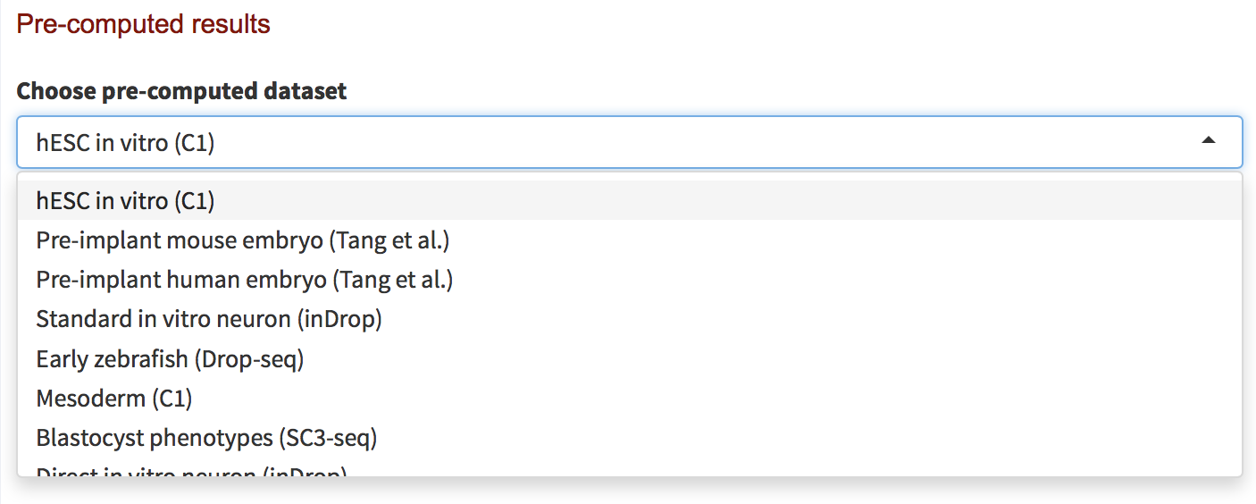
- Click on the bar on the top right side of the page under Pre-computed Datasets.
- You should now see a drop-down menu listing the 42 datasets that have already been analyzed by CytoTRACE. Each dataset is named by biological theme and scRNA-seq platform (e.g. hESC in vitro (C1)), as shown below:
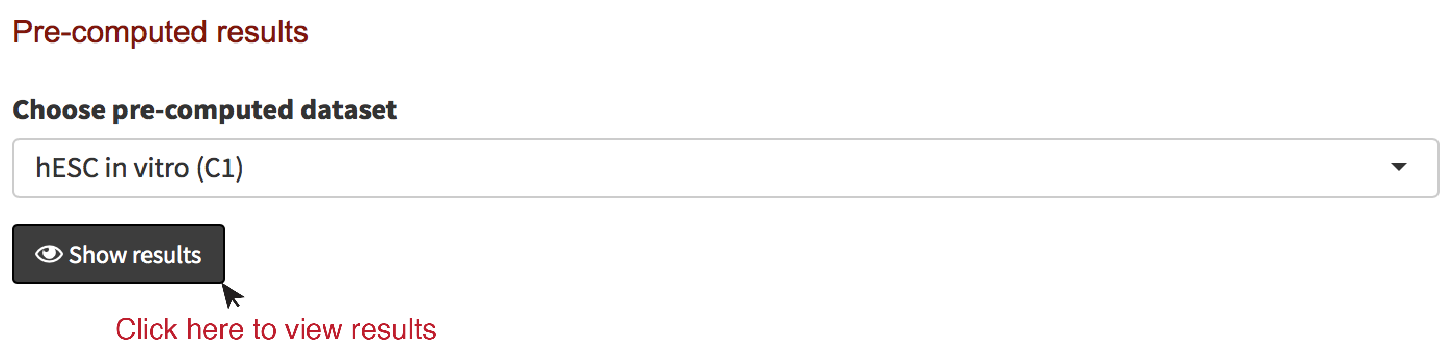
- Once you have selected a dataset to analyze. Click Show results as displayed below.
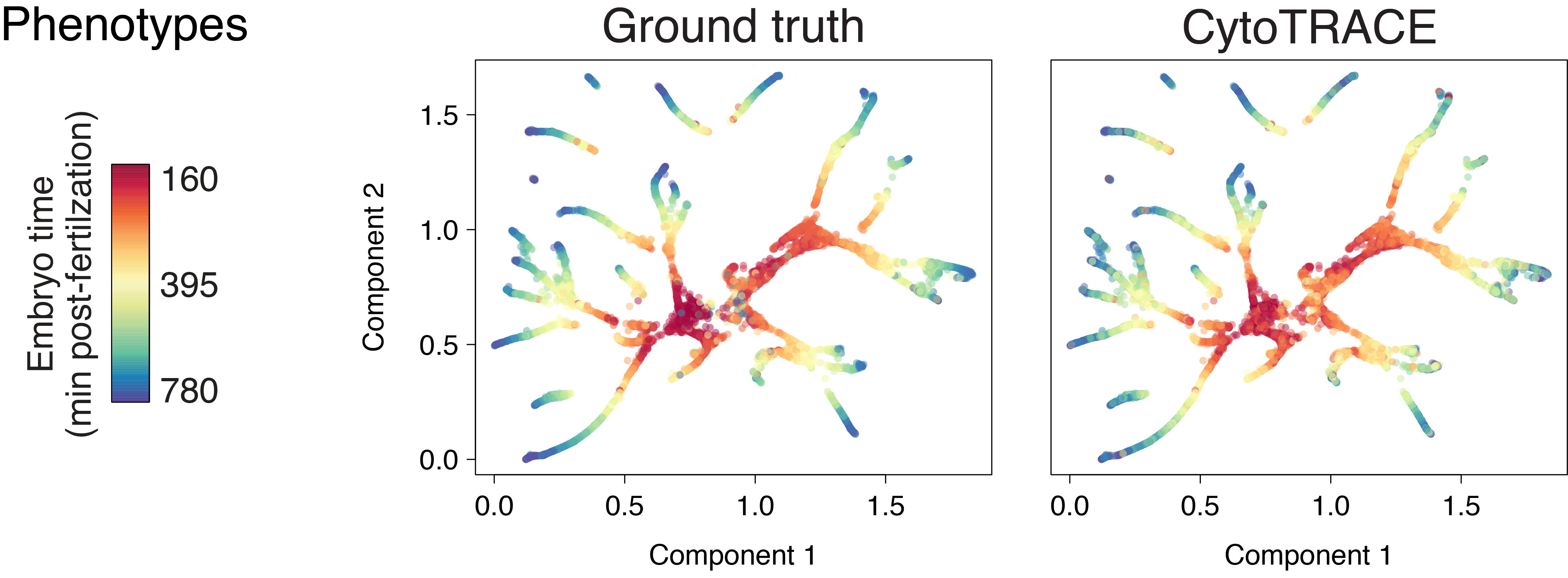
Analyze results I: Low-dimensional visualization
- A useful way to analyze scRNA-seq data is by visualizing a low-dimensional embedding of the data
- We provide two options for visualizing scRNA-seq data:
- 2D visualization
- 3D visualization
- We also provide three options for dimensional reduction:
- t-Distributed Stochastic Neighbor Embedding (t-SNE) with Rtsne (R package)
- Force Atlas 2 with fa2 (Python package)
- Uniform Manifold Approximation and Projection (UMAP) with umap (Python package)
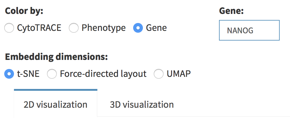
- We also provide three options for the color embeddings:
- CytoTRACE values
- Phenotypes (if provided)
- Gene symbol
- One can toggle between these options using the menu at the top-left of the page
- A 2D example of t-SNE representation of the hESC in vitro (C1) dataset colored by CytoTRACE and phenotype:
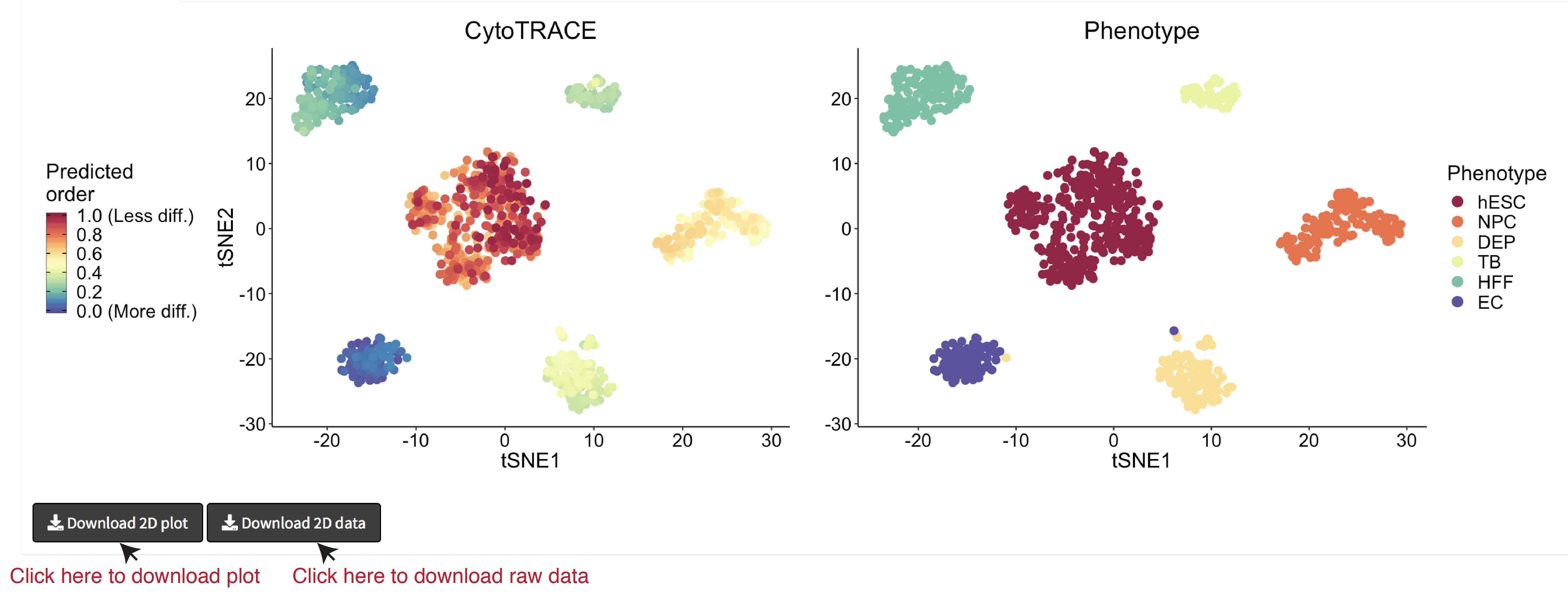
- A 2D example of t-SNE representation of the hESC in vitro (C1) dataset colored by CytoTRACE and NANOG gene expression
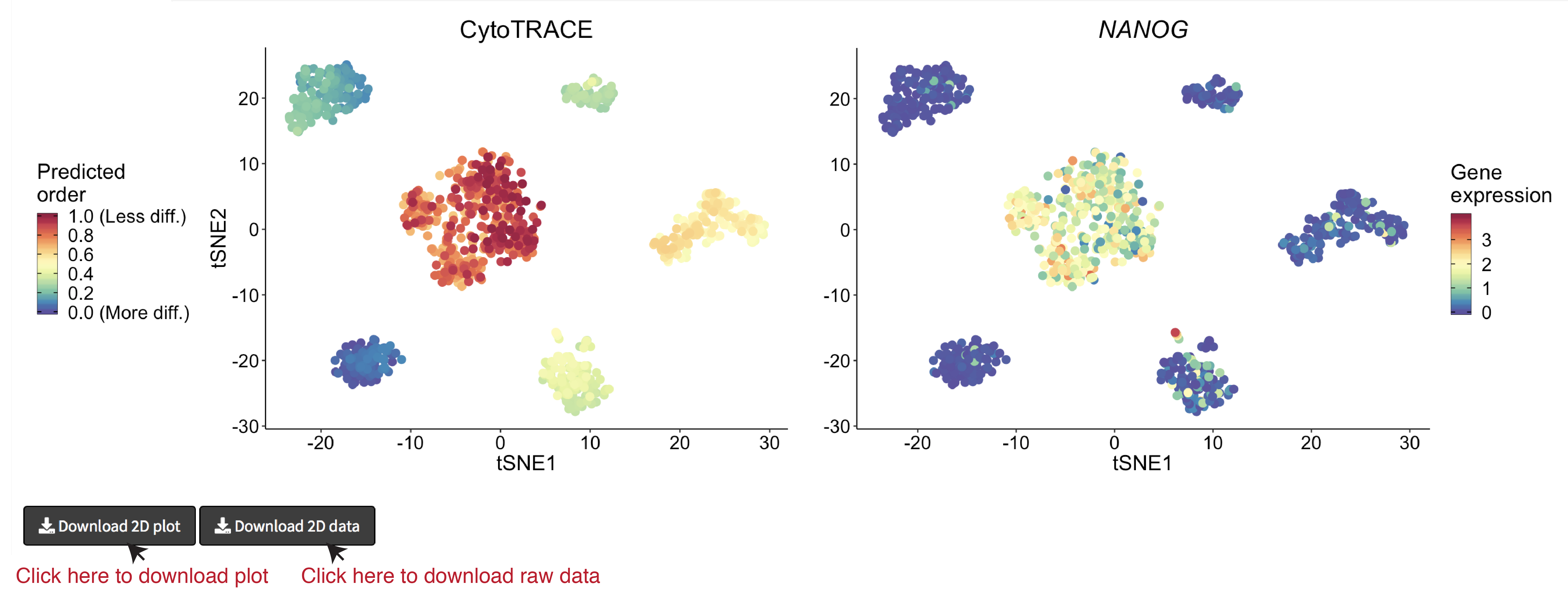
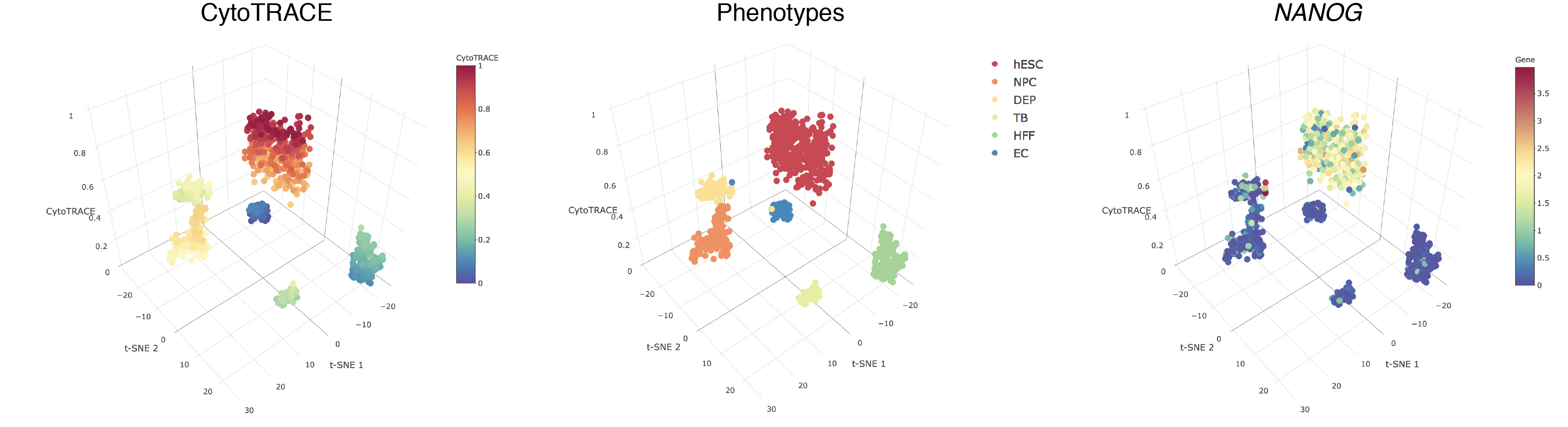
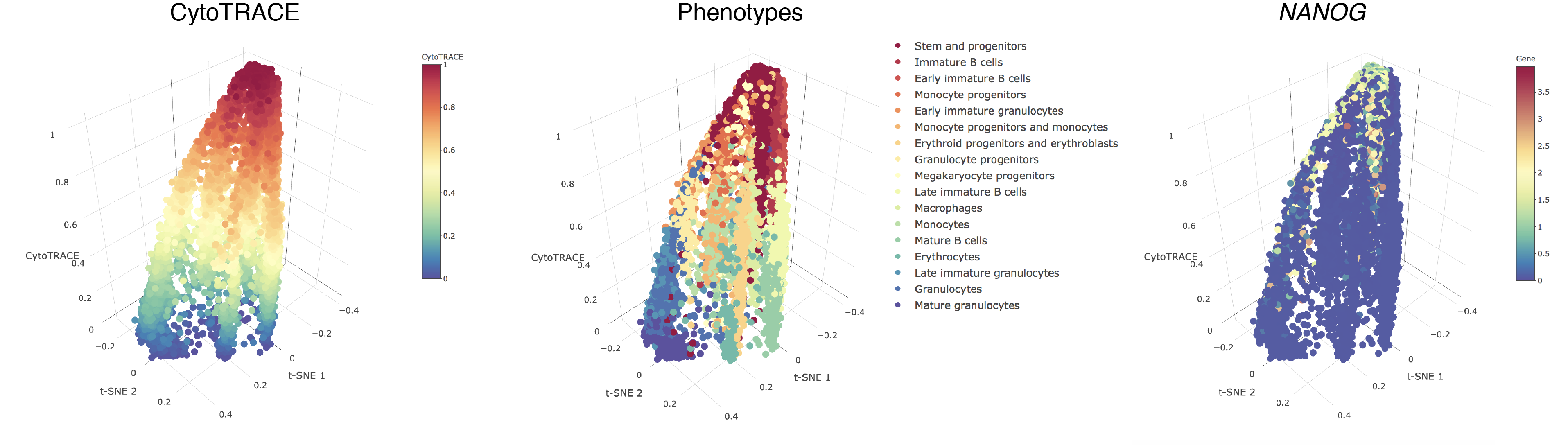
- A 3D example of t-SNE representation of the hESC in vitro (C1) dataset colored by CytoTRACE, phenotype, and NANOG gene expression:
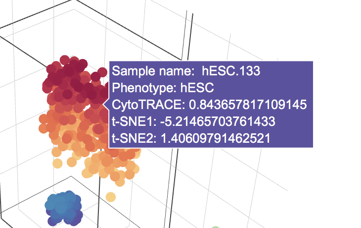
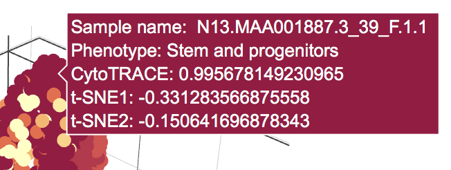
- Hovering over the cells will display a box detailing the sample name, t-SNE coordinates, CytoTRACE value, and phenotype (if provided):
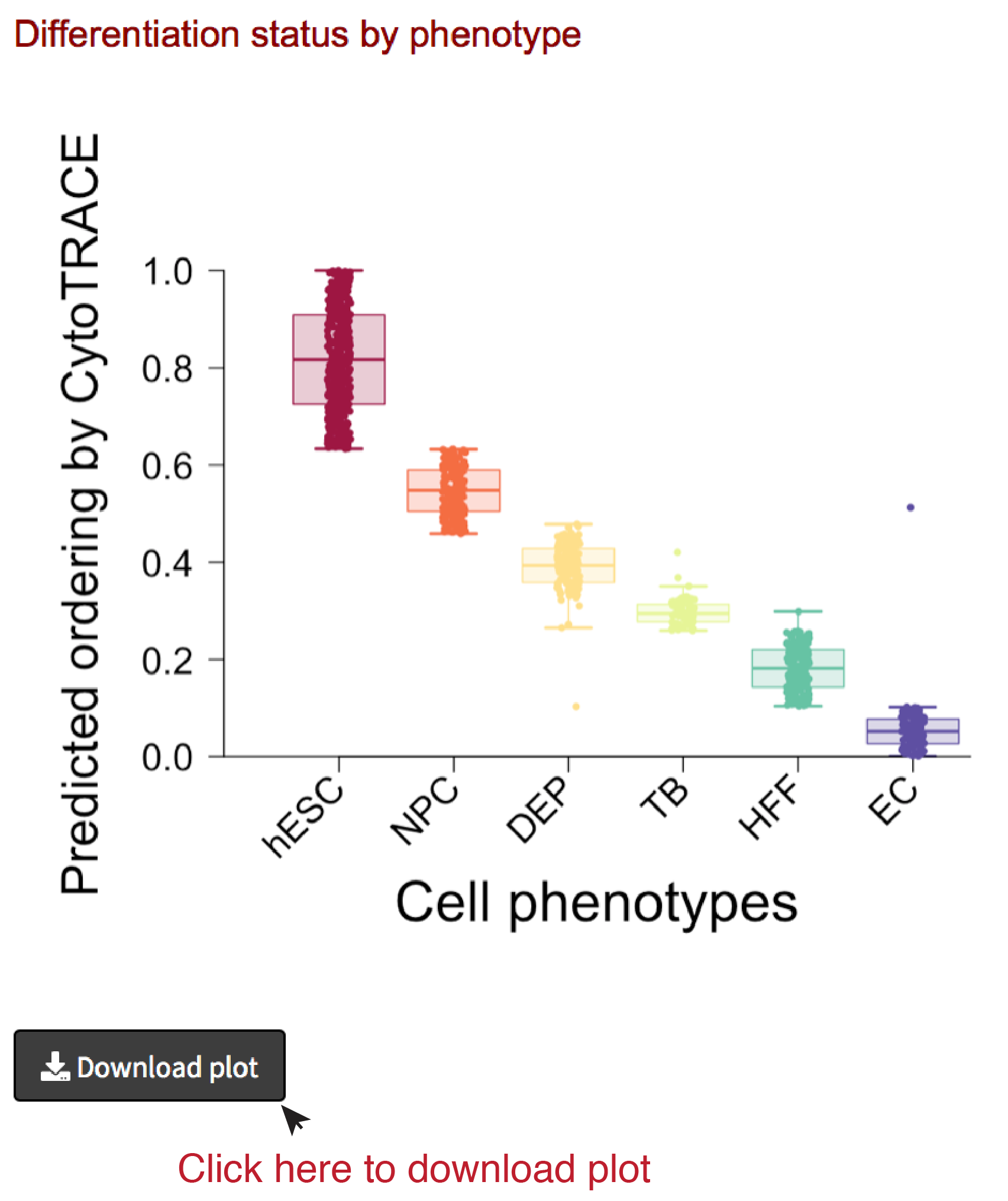
Analyze results II: CytoTRACE by phenotype
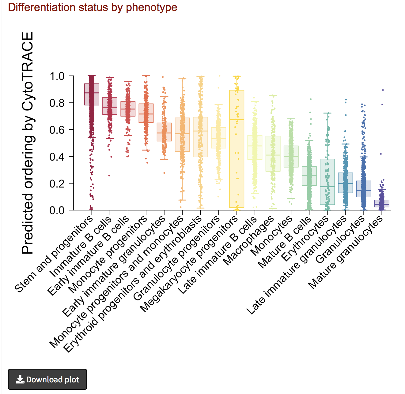
- If phenotype labels are available for each single cell, we can summarize the median and distribution of CytoTRACE values per phenotype using boxplots.
- The boxplot can be downloaded as PDF document by clicking the Download plot button on the bottom left.
Analyze results III: Genes associated with CytoTRACE
- Genes associated with stemness and differentiation can be predicted based on their correlation with CytoTRACE
- The following barplot shows the top 10 (less differentiated; red) and bottom 10 (most differentiated; blue) genes in this dataset based on their correlation with CytoTRACE
- The barplot can be downloaded as a PDF document by clicking the Download plot button in the bottom left.
- The correlation of every provided gene with CytoTRACE can also be downloaded by clicking the Download gene correlations button in the bottom left.
Brief overview
In this tutorial, we provide instructions to analyze a custom single-cell RNA-sequencing (scRNA-seq) dataset. Users have the option to provide phenotype labels for each single cell and perform simple batch correction with ComBat (for integration of multiple complex batches and datasets, see the Scanorama-based implementation under the tab Custom integrated CytoTRACE). For the analysis of multiple and large datasets (e.g. >15,000 cells), we request users to run the R impementation of CytoTRACE (R package).
Please follow the instructions on the tabs above to analyze pre-computed datasets.
Data format
Gene expression table (required)
CytoTRACE takes as input a scRNA-seq gene expression table with the following formatting requirements:
- The matrix must be genes (rows) by cells (columns). The first row must contain the single cell IDs and the first column must contain the gene names.
- The data must be delimited by either commas, tabs, spaces, or semicolons.
- Please DO NOT mean-normalize the expression data or any other normalization scheme that results in negative values in the matrix. Log2-normalized data are accepted, as are data normalized by TPM, FPKM, or RPKM.
- Please DO NOT pre-filter the genes in the expression matrix.
Phenotype table (optional)
Users can choose to provide phenotype labels corresponding to the single cell IDs in the gene expression matrix. Please prepare the phenotype table in the following format:
- The table should contain two columns, where column 1 contains the single cell IDs corresponding to the columns of the scRNA-seq matrix and column 2 contains the corresponding phenotype labels
- Please DO NOT include headers in this table.
Batch (optional)
Users can also choose to provide batch labels corresponding to the single cell IDs in the gene expression matrix. This will be used to correct technical batches with ComBat. For integration of multiple complex batches or datasets, we recommend running CytoTRACE with the Scanorama-based implementation under the tab Custom integrated CytoTRACE. Otherwise, please prepare the batch table in the following format:
- The table should contain two columns, where column 1 contains the single cell IDs corresponding to the columns of the scRNA-seq matrix and column 2 contains the corresponding batch labels
- Please DO NOT include headers in this table.
Example files for trial run
The following data are available for you to download and test-drive CytoTRACE on the website:
Gene expression tables
Phenotype tables
Upload data
Select your CytoTRACE run mode
- Indicate whether or not you want to apply CytoTRACE on a single dataset or across multiple datasets by integration. For this tutorial, we will run CytoTRACE on a single dataset without dataset integration (default). For information on how to run CytoTRACE on multiple datasets with Scanorma-based integration, please read the tutorial, Custom integrated CytoTRACE
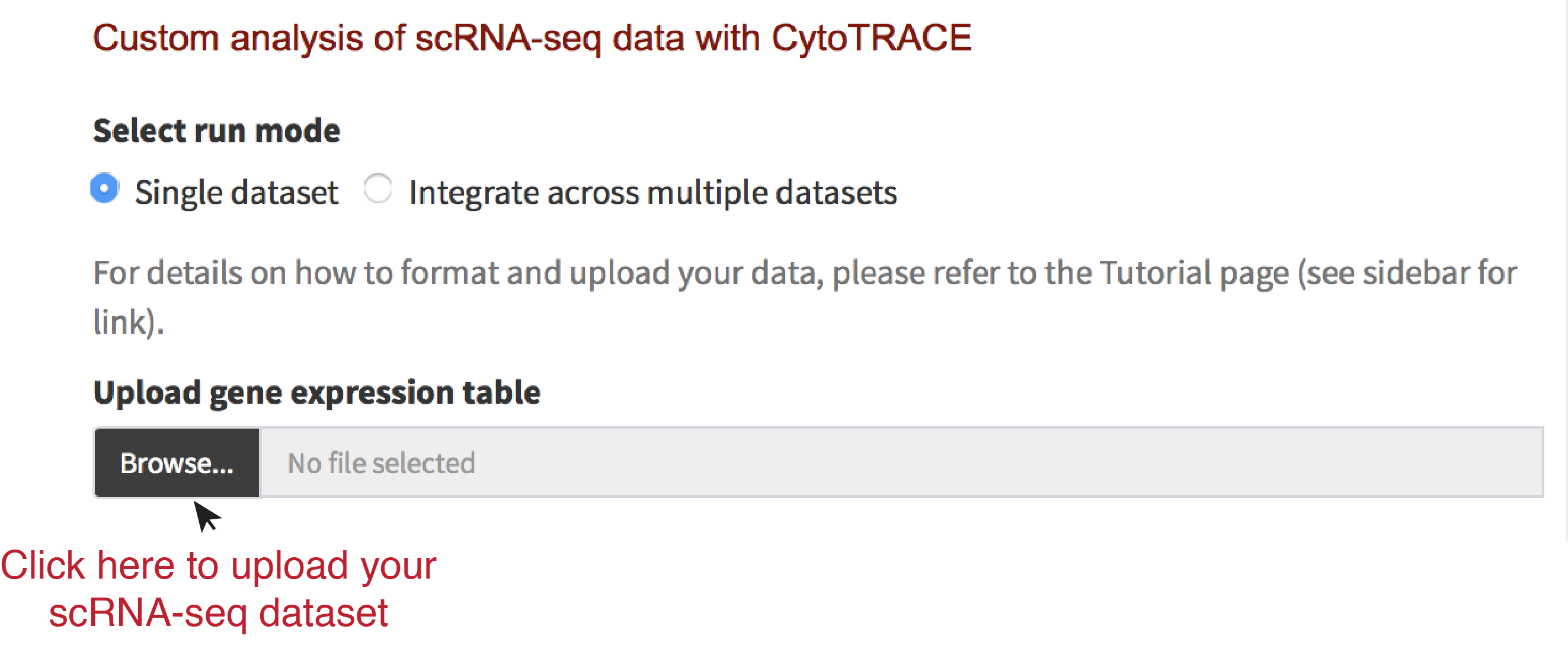
Upload your gene expression table (required)
- After formatting your gene expression table as instructed in the Setup tab, click the Browse button to upload your data.
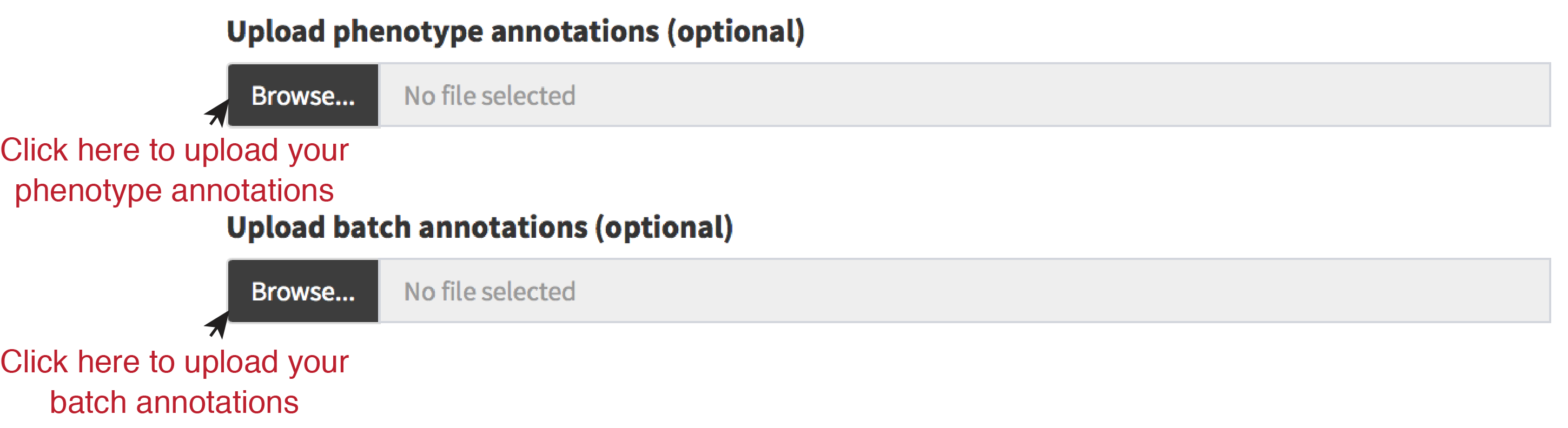
Upload your phenotype and batch tables (optional)
- Once the expression table has been uploaded, the option to upload phenotype and batch data will be provided.
- After formatting your tables as instructed in the Setup tab, click the Browse button to upload your data.
Run CytoTRACE
After uploading all your files, click Run CytoTRACE. Running CytoTRACE may take some time with large datasets. Once the analysis is complete, you will be directed to a another page with the results of your run. These are detailed in the next three tabs.

Analyze results I: Low-dimensional visualization
- A useful way to analyze scRNA-seq data is by visualizing a low-dimensional embedding of the data
- We provide two options for visualizing scRNA-seq data:
- 2D visualization
- 3D visualization
- We also provide three options for dimensional reduction:
- t-Distributed Stochastic Neighbor Embedding (t-SNE) with Rtsne (R package)
- Force Atlas 2 with fa2 (Python package)
- Uniform Manifold Approximation and Projection (UMAP) with umap (Python package)
- We also provide three options for the color embeddings:
- CytoTRACE values
- Phenotypes (if provided)
- Gene symbol
- One can toggle between these options using the menu at the top-left of the page
- A 2D example of t-SNE representation of the hESC in vitro (C1) dataset colored by CytoTRACE and phenotype:
- A 2D example of t-SNE representation of the hESC in vitro (C1) dataset colored by CytoTRACE and NANOG gene expression
- A 3D example of t-SNE representation of the hESC in vitro (C1) dataset colored by CytoTRACE, phenotype, and NANOG gene expression:
- Hovering over the cells will display a box detailing the sample name, t-SNE coordinates, CytoTRACE value, and phenotype (if provided):
Analyze results II: CytoTRACE by phenotype
- If phenotype labels are available for each single cell, we can summarize the median and distribution of CytoTRACE values per phenotype using boxplots.
- The boxplot can be downloaded as PDF document by clicking the Download plot button on the bottom left.
Analyze results III: Genes associated with CytoTRACE
- Genes associated with stemness and differentiation can be predicted based on their correlation with CytoTRACE
- The following barplot shows the top 10 (less differentiated; red) and bottom 10 (most differentiated; blue) genes in this dataset based on their correlation with CytoTRACE
- The barplot can be downloaded as a PDF document by clicking the Download plot button in the bottom left.
- The correlation of every provided gene with CytoTRACE can also be downloaded by clicking the Download gene correlations button in the bottom left.
Brief overview
In this tutorial, we provide instructions to calculate CytoTRACE values across multiple heterogeneous single-cell RNA-sequencing (scRNA-seq) datasets using a Scanorama-based implementation. Currently, the website implementation is limited to the integration of up to 5 datasets. For integration of more than 5 datasets, especially when the number of total cells exceed 15,000, we request users to run the R implementation of integrated CytoTRACE (iCytoTRACE function in R package; see Install R package in the sidebar).
Please follow the instructions on the right to integrate and calculate CytoTRACE across your custom scRNA-seq datasets..
Data format
Gene expression tables (required)
integrated CytoTRACE (iCytoTRACE) takes as input at least two scRNA-seq gene expression tables with the following formatting requirements:
- The matrices must be genes (rows) by cells (columns). The first row must contain the single cell IDs and the first column must contain the gene names.
- The data must be delimited by either commas, tabs, spaces, or semicolons.
- Please DO NOT mean-normalize the expression data or any other normalization scheme that results in negative values in the matrix. Log2-normalized data are accepted, as are data normalized by TPM, FPKM, or RPKM.
- Please DO NOT pre-filter the genes in the expression matrix.
- Datasets must have at least one cell population shared among pairs of datasets. Please refer to the original Scanorama manuscript for further details
(Hie et al., 2019).
Phenotype tables (optional)
Users can choose to provide phenotype labels corresponding to the single cell IDs in the gene expression matrices. Please prepare the phenotype table in the following format:
- The tables should contain two columns, where column 1 contains the single cell IDs corresponding to the columns of the scRNA-seq matrix and column 2 contains the corresponding phenotype labels
- Please DO NOT include headers in this table.
Example files for trial run
The following data are available for you to download and test-drive iCytoTRACE on the website:
Gene expression tables
- scRNA-seq dataset of bone marrow differentiation (10x)
- scRNA-seq dataset of bone marrow differentiation (Smart-seq2)
Phenotype tables
Upload data
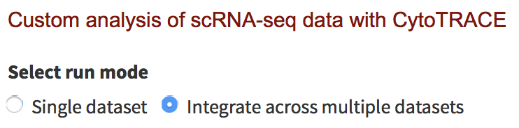
Select your CytoTRACE run mode
- Indicate whether or not you want to apply iCytoTRACE on a single dataset or across multiple datasets by integration. For this tutorial, we will run iCytoTRACE on multiple datasets by integration (default). For information on how to run iCytoTRACE on a single dataset, please read the tutorial, Analyze a custom scRNA-seq dataset
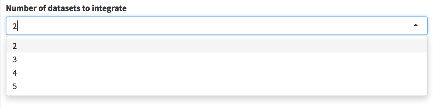
Select the number of datasets you wish to integrate
- Please select up to 5 datasets for the integrated iCytoTRACE run
- For integration of more than 5 datasets, especially when total cell numbers exceed 15,000 single cells, we request users to run the R implementation of integrated CytoTRACE (iCytoTRACE function in R package).
Upload your gene expression table (required) and phenotype tables (optional)
- After indicating the number of datasets, new fields will appear on the right side of the page for you to upload your data.
- After formatting your gene expression and phenotype tables as instructed in the Setup tab, click the Browse button to upload your data in the respective fields.
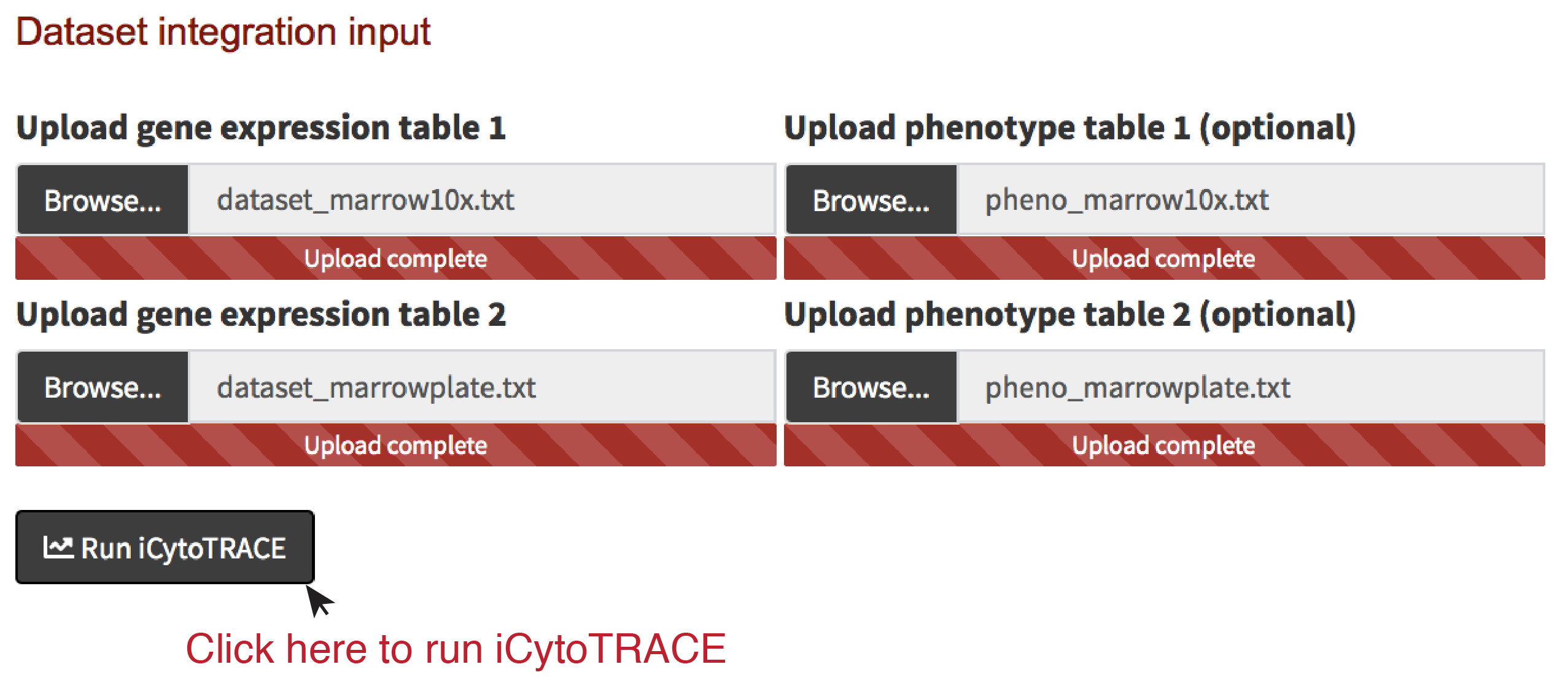
Run iCytoTRACE
After uploading all your files, click Run iCytoTRACE (see above). Running iCytoTRACE may take some time with multiple large datasets. Once the analysis is complete, you will be directed to a another page with the results of your run. These are detailed in the next three tabs.
Analyze results I: Low-dimensional visualization
- A useful way to analyze scRNA-seq data is by visualizing a low-dimensional embedding of the data
- We use the low-dimensional t-SNE embeddings outputted from Scanorama (Python package) to visualize integrated datasets
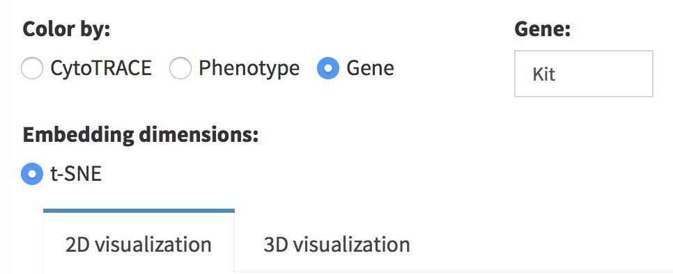
- We also provide three options for the color embeddings:
- CytoTRACE values
- Phenotypes (if provided)
- Gene symbol
Analyze results I: Low-dimensional visualization
- A useful way to analyze scRNA-seq data is by visualizing a low-dimensional embedding of the data
- We provide two options for visualizing scRNA-seq data:
- 2D visualization
- 3D visualization
- We also provide three options for dimensional reduction:
- t-Distributed Stochastic Neighbor Embedding (t-SNE) with Rtsne (R package)
- Force Atlas 2 with fa2 (Python package)
- Uniform Manifold Approximation and Projection (UMAP) with umap (Python package)
- We also provide three options for the color embeddings:
- CytoTRACE values
- Phenotypes (if provided)
- Gene symbol
- One can toggle between these options using the menu at the top-left of the page
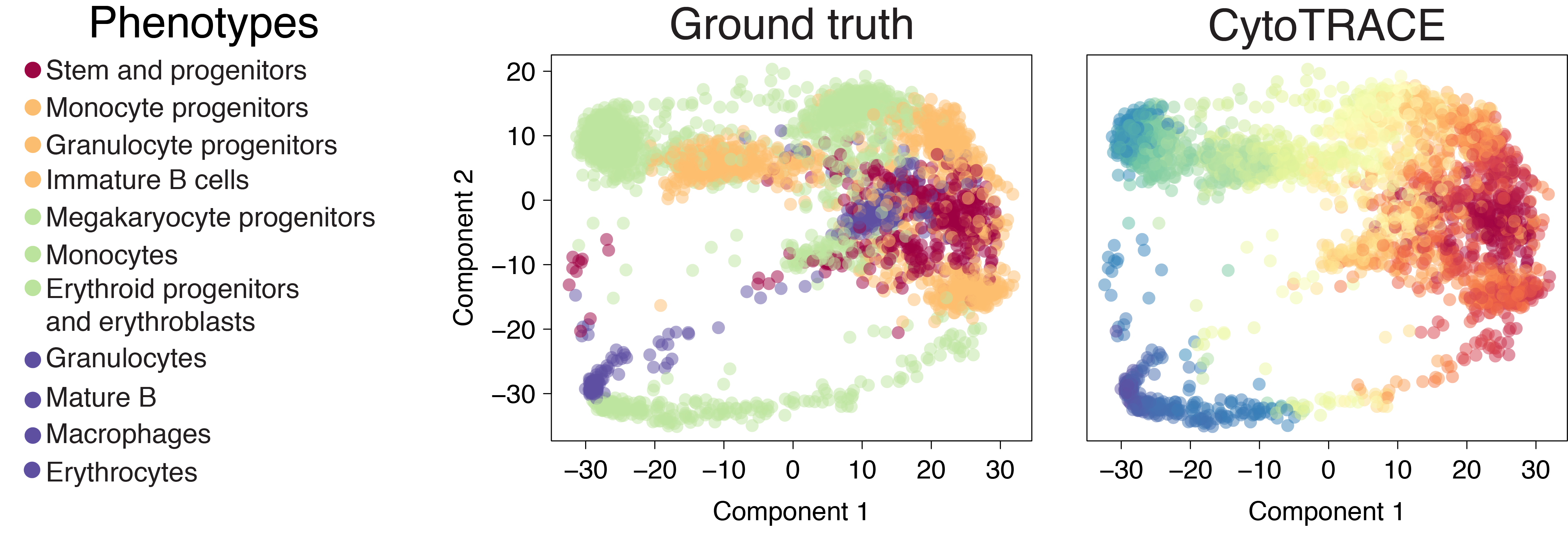
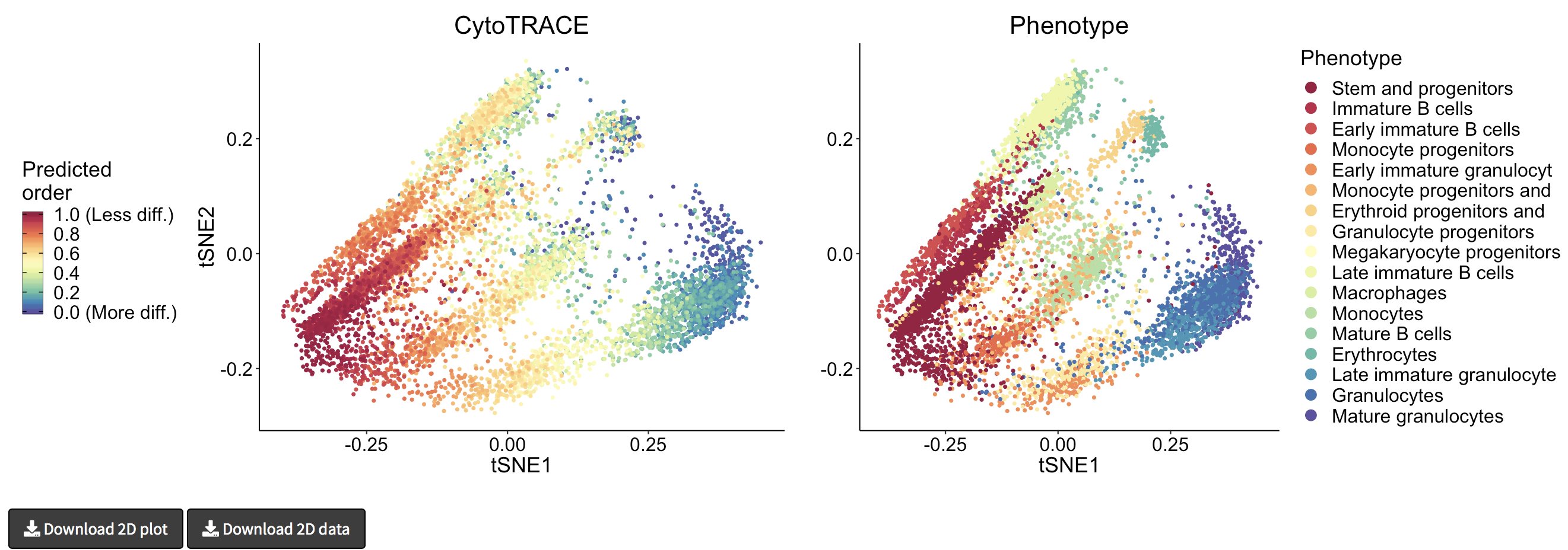
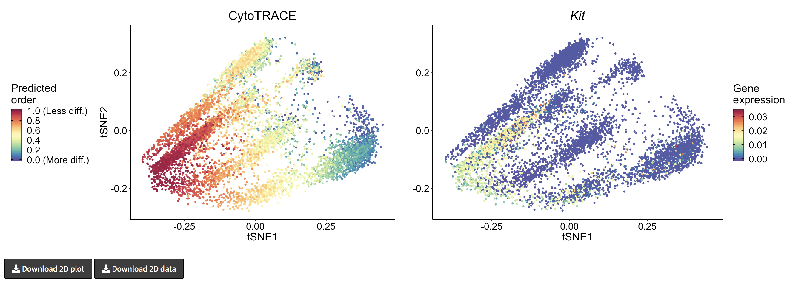
- A 2D example of t-SNE representation of the Bone marrow (Smart-seq2) dataset colored by CytoTRACE and phenotype:
- A 2D example of t-SNE representation of the Bone marrow (Smart-seq2) dataset colored by CytoTRACE and Kit gene expression
- A 3D example of t-SNE representation of the Bone marrow (Smart-seq2) dataset colored by CytoTRACE, phenotype, and Kit gene expression:
- Hovering over the cells will display a box detailing the sample name, t-SNE coordinates, CytoTRACE value, and phenotype (if provided):
Analyze results II: iCytoTRACE by phenotype
- If phenotype labels are available for each single cell, we can summarize the median and distribution of iCytoTRACE values per phenotype using boxplots.
- The boxplot can be downloaded as PDF document by clicking the Download plot button on the bottom left.
Analyze results III: Genes associated with iCytoTRACE
- Genes associated with stemness and differentiation can be predicted based on their correlation with iCytoTRACE
- The following barplot shows the top 10 stemness (red) and differentiation-associated (blue) genes in this dataset based on their correlation with iCytoTRACE
- The barplot can be downloaded as PDF document by clicking the Download plot button in the bottom left.
- The correlation of every provided gene with iCytoTRACE can also be downloaded by clicking the Download gene ordering button in the bottom left.
Characterization of molecular themes
To understand the molecular themes prioritized by gene counts across different datasets, we analyzed the assocation between known molecular signatures (e.g. 17,810 gene sets from MSigDB and 896 gene sets of TF binding sites from ENCODE/ChEA) and the genes associated with gene counts. To do this, we performed single sample gene set enrichment analysis (ssGSEA) on a gene list ordered by the Pearson correlation between log2 gene expression and gene counts from each dataset and report the normalized enrichment score (NES) for the 18,706 known molecular signatures.
License agreement
1. The Board of Trustees of the Leland Stanford Junior University (“Stanford”) provides CytoTRACE software and code (“Service”) free of charge for non-commercial use only. Use of the Service by any commercial entity for any purpose, including research, is prohibited.
2. By using the Service, you agree to be bound by the terms of this Agreement. Please read it carefully.
3. You agree not to use the Service for commercial advantage, or in the course of for-profit activities. You agree not to use the Service on behalf of any organization that is not a non-profit organization. Commercial entities wishing to use this Service should contact Stanford University’s Office of Technology Licensing and reference docket S18-500.
4. THE SERVICE IS OFFERED “AS IS”, AND, TO THE EXTENT PERMITTED BY LAW, STANFORD MAKES NO REPRESENTATIONS AND EXTENDS NO WARRANTIES OF ANY KIND, EITHER EXPRESS OR IMPLIED. STANFORD SHALL NOT BE LIABLE FOR ANY CLAIMS OR DAMAGES WITH RESPECT TO ANY LOSS OR OTHER CLAIM BY YOU OR ANY THIRD PARTY ON ACCOUNT OF, OR ARISING FROM THE USE OF THE SERVICE. YOU HEREBY AGREE TO DEFEND AND INDEMNIFY STANFORD, ITS TRUSTEES, EMPLOYEES, OFFICERS, STUDENTS, AGENTS, FACULTY, REPRESENTATIVES, AND VOLUNTEERS (“STANFORD INDEMNITEES”) FROM ANY LOSS OR CLAIM ASSERTED AGAINST STANFORD INDEMNITEES ARISING FROM YOUR USE OF THE SERVICE.
5. All rights not expressly granted to you in this Agreement are reserved and retained by Stanford or its licensors or content providers. This Agreement provides no license under any patent.
6. You agree that this Agreement and any dispute arising under it is governed by the laws of the State of California, United States of America, applicable to agreements negotiated, executed, and performed within California.
7. Subject to your compliance with the terms and conditions set forth in this Agreement, Stanford grants you a revocable, non-exclusive, non-transferable right to access and make use of the Service.
Do you accept the terms and conditions in this agreement?